Data Mining Survivor: Getting_Started - Our First Model--Some Details

The file weather.csv has been read as a dataset. Formally the object within R is known as a data frame. We are now ready to build a model or two.

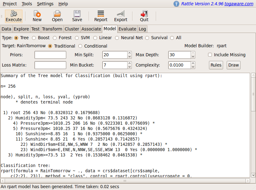
Using Rattle we simply click the Model tab to be presented with the Model options we see in Figure 2.4. To build a decision tree model, one of the most common data mining models, simply click the Execute button to obtain the textual representation of the model shown in Figure 2.4.

**Figure 2.4:** The `weather` dataset has been loaded and a decision tree model has been built.

The target variable is RainTomorrow, as we would see if we were to scroll the Data tab window in Figure 2.3. Using the weather dataset our modelling task is to learn about the prospects of it raining tomorrow, given what we know about today. The model, represented textually, can be seen in Figure 2.4. We can also view the same text in the R console:

> print(crs$rpart, digits = 1)

n= 256 

node), split, n, loss, yval, (yprob)
      * denotes terminal node

 1) root 256 40 No (0.83 0.17)  
   2) Humidity3pm< 7e+01 243 30 No (0.87 0.13)  
     4) Pressure3pm>=1e+03 206 20 No (0.92 0.08) *
     5) Pressure3pm< 1e+03 37 20 No (0.57 0.43)  
      10) Sunshine>=9 16  1 No (0.94 0.06) *
      11) Sunshine< 9 21  6 Yes (0.29 0.71)  
        22) WindDir9am=ESE,NW,S,WNW 7  2 No (0.71 0.29) *
        23) WindDir9am=E,ENE,N,NNW,SE,SSE,WSW 13  0 Yes (0.00 1.00) *
   3) Humidity3pm>=7e+01 13  2 Yes (0.15 0.85) *

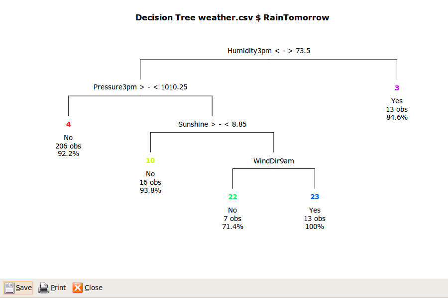
The textual presentation (as above or in Figure 2.4) will take a little effort to understand and it is fully explained in Chapter

. For now we might click on the Draw button provided by Rattle for a picture of the decision tree, to obtain the plot that we see in Figure 2.5. The plot provides a better idea of why it is called a decision tree.

**Figure 2.5:** The decision tree built ``out of the box'' with Rattle. We traverse the tree by following the branches corresponding to the tests at each node. The leaf nodes include a node number for reference, a decision of 0 or 1 to indicate whether it will RainTomorrow, the number of training observations and the strength or confidence of the decision.

Now click on the Rules button to obtain a list of rules that are derived directly from the decision tree (we'll need to scroll down the textview of the model tab). The R command that Rattle provides to list the rules is the function Rfunction[]asRules:

> asRules(crs$rpart)

 Rule number: 23 [yval=Yes cover=13 (5%) prob=1.00]
   Humidity3pm< 73.5
   Pressure3pm< 1010
   Sunshine< 8.85
   WindDir9am=E,ENE,N,NNW,SE,SSE,WSW

 Rule number: 3 [yval=Yes cover=13 (5%) prob=0.85]
   Humidity3pm>=73.5

 Rule number: 22 [yval=No cover=7 (3%) prob=0.29]
   Humidity3pm< 73.5
   Pressure3pm< 1010
   Sunshine< 8.85
   WindDir9am=ESE,NW,S,WNW

 Rule number: 4 [yval=No cover=206 (80%) prob=0.08]
   Humidity3pm< 73.5
   Pressure3pm>=1010

 Rule number: 10 [yval=No cover=16 (6%) prob=0.06]
   Humidity3pm< 73.5
   Pressure3pm< 1010
   Sunshine>=8.85

A well recognised advantage of the decision tree representation of a model is that the paths through the decision tree can be interpreted as a collection of rules, as we have just seen. The rules are perhaps somewhat more readable. They are listed in the order of their strength in predicting the target variable (will it rain tomorrow?). Thus, rule number 23 (which also corresponds to the 23) in Figure 2.4 and node number 23 in Figure 2.5) is the strongest rule predicting rain. We can read it as saying that if the humidity at 3pm is less than 73.5, and the atmospheric pressure (reduced to mean sea level) at 3pm is less than 1010 hectopascals, and the amount of sunshine today was less than 8.85, and the wind direction at 9am was one of E, ENE, N, NNW, SE, SSE, or WSW, then it seems there is a pretty good chance of rain tomorrow. That is to say, every time we see these conditions in the past (represented in the data) it has always rained tomorrow. I would take my umbrella with me.

Progressing down to the other end of the list of rules, rule number 10 tells us that if, instead, the amount of sunshine is greater than or equal to 8.85 (but with the same humidity and pressure conditions at 3pm), then it is less likely to be raining tomorrow (in this case, it suggests only a 6% probability (prob=0.06).

We now have our first model built, data mining our historic observations of weather, to help provide some insight about whether it will rain tomorrow.