
Desktop Survival Guide
by Graham Williams
|
|
DATA MINING
Desktop Survival Guide by Graham Williams |
|
|||
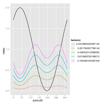
Using GGPlot |


|
> library(ggplot2)
> a <- seq(0, 360, 5)*pi/180
> s <- seq(5, 45, 10)*pi/180
> dataset <- expand.grid(a = a, s = s)
> dataset$ac <- sin(dataset$a + (45*pi/180)) + 1
> dataset$asc <- dataset$s * (cos(dataset$ac) + sin(dataset$ac))
> p <- ggplot(data = dataset, aes(x = a, y = ac)) +
    geom_line() +
    geom_line(aes(y = asc, colour = factor(s))) +
    geom_vline(intercept = c(45, 225)*pi/180) +
    scale_x_continuous("azimuth", breaks = seq(0,6,1), labels=round(seq(0,6,1)*180/pi)) +
    scale_y_continuous("index")
> print(p)
|
Some ``lattice'' plots, not as in the lattice package but in drawing a
lattice graphic.
library(ggplot2) dataset <- expand.grid(x = 1:10, y = 1:50) dataset$z <- runif(nrow(dataset)) ggplot(data = dataset, aes(x = x, y = y, fill = z)) + geom_tile() + scale_fill_gradient(low="white", high="black") + coord_equal() |
library(plotrix) transect<-matrix(runif(1000),nrow=5) x11(width=14,height=2.4) color2D.matplot(transect,c(1,0),c(1,0),c(1,0), main="Shrubbery",show.legend=TRUE) |