Desktop Survival Guide
by Graham Williams
|
|
DATA MINING
Desktop Survival Guide by Graham Williams |
|
|||
Decision Tree |


|
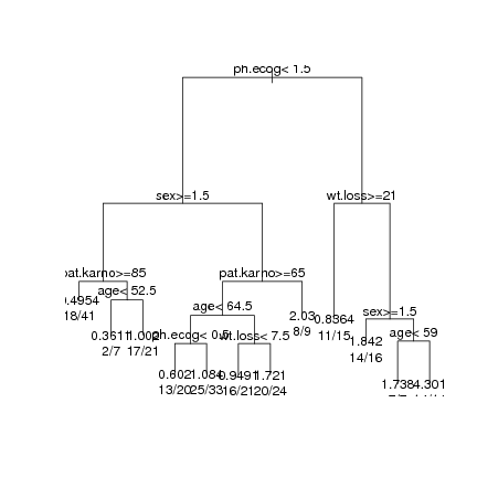
The rpart function can also be used with a Surv object as the target. Here we build a decision tree.
> library(rpart)
> l.rpart <- rpart(l.Surv ~ age + sex + ph.ecog + ph.karno + pat.karno +
                   meal.cal + wt.loss, data=lung)
> l.rpart
|
n= 228

node), split, n, deviance, yval
      * denotes terminal node

 1) root 228 307.928100 1.0000000
   2) ph.ecog< 1.5 176 223.146500 0.8607050
     4) sex>=1.5 69  79.663710 0.6067812
       8) pat.karno>=85 41  38.552160 0.4954413 *
       9) pat.karno< 85 28  38.961790 0.7912681
        18) age< 52.5 7   8.297501 0.3610969 *
        19) age>=52.5 21  26.638230 1.0017890 *
     5) sex< 1.5 107 134.504400 1.0669060
      10) pat.karno>=65 98 123.426900 1.0085900
        20) age< 64.5 53  63.983660 0.8433300
          40) ph.ecog< 0.5 20  22.029470 0.6019784 *
          41) ph.ecog>=0.5 33  38.488990 1.0838490 *
        21) age>=64.5 45  56.194870 1.2707780
          42) wt.loss< 7.5 21  22.817280 0.9491270 *
          43) wt.loss>=7.5 24  29.796110 1.7206300 *
      11) pat.karno< 65 9   7.162132 2.0298660 *
   3) ph.ecog>=1.5 52  70.309440 1.7041700
     6) wt.loss>=21 15  18.094340 0.8363971 *
     7) wt.loss< 21 37  38.904150 2.5294840
      14) sex>=1.5 16   8.883448 1.8424400 *
      15) sex< 1.5 21  27.485660 3.1026240
        30) age< 59 7   4.587466 1.7378480 *
        31) age>=59 14  17.993450 4.3012260 *
|
The summary command will provide fuller details of the resulting model.
> summary(l.rpart) |
The usual predict can be used to obtain the predictions of the estimated rate. Todo: What is actually being predicted here? These are compared to the same predictions from the coxph model.
> l.rpart.pred <- predict(l.rpart, lung) > results <- cbind(l.coxph.age.results, rpart=l.rpart.pred) > head(results) |
  time status        lp     risk  expected       sex
1  306      2 0.2096146 1.233203 0.8280030 0.2096146
2  455      2 0.2096146 1.233203 1.3880051 0.2096146
3 1010      1 0.2096146 1.233203 3.5060567 0.2096146
4  210      2 0.2096146 1.233203 0.5185439 0.2096146
5  883      2 0.2096146 1.233203 3.5060567 0.2096146
6 1022      1 0.2096146 1.233203 3.5060567 0.2096146
      rpart
1 0.9491270
2 1.7206297
3 0.6019784
4 2.0298656
5 0.6019784
6 0.9491270
|
> plot(l.rpart) > text(l.rpart, use.n=TRUE) |