DATA MINING Desktop Survival Guide by Graham Williams
Desktop Survival Project Home Introduction Getting Started The Business Problem Data Loading Data Exploring Data Interactive Graphics Test Models Text Mining Decision Trees Forests Support Vector Machine Linear Regression Neural Network Naive Bayes Survival Analysis Evaluation and Deployment Data Cleaning Handling Missing Data Transforming Data Data Reduction Deployment Troubleshooting Issues Moving into R R Getting Help Data Graphics in R Understanding Data Preparing Data Issues Evaluating Models Reporting Fraud Analysis Archetype Analysis Algorithms Bayes Classifier K-Nearest Neighbours Linear Models Open Products AlphaMiner Borgelt Data Mining Suite KNime R Rattle Weka Closed Products Clementine Equbits Foresight GhostMiner InductionEngine ODM Enterprise Miner Statistica Data Miner TreeNet Virtual Predict Installing Rattle Projects Bibliography Index Preface Goals Organisation Features Audience Typographical Conventions A Note on Languages Currency Acknowledgements Introduction Data Mining The Business Problem Types of Analysis Data Mining Applications A Framework for Modelling Agile Data Mining R Rattle Why R and Rattle? Data Preparation Number of Algorithms Repeatability Performance Open Source Data Mining Business Case Sample Business Case Pros and Cons Books on R Getting Started Initial Interaction with R Quitting Rattle and R First Contact Loading a Dataset Building a Model Understanding Our Data Evaluating the Model Evaluating the Model Interacting with R Interacting with Rattle Projects Toolbar Menus Interacting with Plots Keyboard Navigation Summary Command Summary The Business Problem Solar Panel Efficiency Water Collection Others Other Business Problems Fraud Detection Loan Approval Documenting the Business Problem Review Further Resources Chapter Exercises Data Data Nomenclature Loading Data into Rattle CSV Data Datasets Reading Direct from URL Play Golf Weather Data Other Data Sources ARFF Data ODBC Sourced Data Setting Up a Data Source Name Netezza Setup Teradata Setup R Data R Dataset Data Entry Data Tab Options in Rattle Sampling Data Variable Roles Automatic Role Identification Weights Calculator Manipulating Data Loading Data CSV Data Locating and Loading Data Loading the File CSV Options Basic Data Summary ARFF Data ODBC Sourced Data R Dataset R Data Library Data Options Sampling Data Variable Roles Automatic Role Identification Weights Calculator Command Summary Exploring Data Summarising Data Summary Describe Basics Kurtosis Skewness Missing Exploring Distributions Box Plot Histogram Cumulative Distribution Plot Benford's Law Other Digits Stratified Benford Plots Bar Plot Dot Plot Mosaic Plot GGobi Scatterplot Data Viewer Brushing Identify Multivariate Outliers Other Options Quality Plots Using R Further GGobi Documentation Correlation Analysis Hierarchical Correlation Principal Components Single Variable Overviews Interactive Graphics Interactive Visualisations Latticist GGobi Scatterplot Multiple Plots Brushing Other Plots Data Viewer Brushing Identify Multivariate Outliers Other Options Quality Plots Using R Further GGobi Documentation Documenting Interactive Explorations Code Review Chapter Exercises Command Summary Test Models A Framework for Modelling Descriptive Analytics Predictive Analytics Documenting Models Summary Code Review Exercises Further Resources Command Summary Cluster Analysis Summary Clusters Basic Clustering Hot Spots Alternative Clustering Other Cluster Examples KMeans Export KMeans Clusters Discriminant Coordinates Plot Number of Clusters Hierarchical Clusters Other Cluster Algorithms Association Analysis Summary Overview Algorithm Usage Read Transactions file format sep cols rm.duplicates Summary Apriori data parameter appearance control Inspect Examples Video Marketing Survey Data Other Examples Resources and Further Reading Basket Analysis General Rules Network Analysis Documenting Interactive Explorations Code Review Chapter Exercises Command Summary Text Mining Application to Text Text Mining with R Decision Trees Knowledge Representation Search Heuristic Measures Tutorial Example Rattle R Tuning Parameters Min Split (Rarg[]minsplit) Min Bucket (minbucket) Priors (prior) Loss Matrix Complexity (cp) Other Options Simple Example Convert Tree to Rules Predicting Salary Group Issues Summary Code Review Iris Wine Exercises Resources Command Summary Forests Knowledge Representation Algorithm Boosting Random Forest Measures Tutorial Example Rattle Boosting Random Forest R Boosting Step by Step Using gbm Random Forest Tutorial Example Tuning Parameters Boosting Random Forest Tuning Parameters Number of Trees Sample Size Number of Variables Random Forest importance classwt Examples Summary Random Forest Code Review Resources Boosting Random Forests Bagging Exercises Command Summary Support Vector Machine Formalities Tutorial Example Tuning parameters Examples Resources and Further Reading Overview Examples Resources and Further Reading Linear Regression Linear Regression Formalities Tutorial Example Tuning parameters Generalized Regression Formalities Tutorial Example Tuning parameters Logistic Regression Formalities Tutorial Example Tuning parameters Discussion Probit Regression Formalities Tutorial Example Tuning Parameters Multinomial Regression Formalities Tutorial Example Tuning Parameters Neural Network Formalities Tutorial Example Tuning parameters Documenting Code Review Further Resources Chapter Exercises Command Summary Naive Bayes Summary Code Review Resources Exercises Command Summary Survival Analysis Sample Data Simple Lung Descriptive Analysis Regression survreg Simple Lung coxph Simple Lung Apply to New Data More Input Variables Decision Tree Example from Singer and Willett Other Approaches Design Package Random Survival Forests Prediction on Test Data Evaluation The Evaluate Tab Confusion Matrix Measures Graphical Measures Risk Charts Cost Curves Lift ROC Curves Area Under Curve Precision versus Recall Sensitivity versus Specificity Predicted versus Observed Scoring Documenting Interactive Explorations Code Review Chapter Exercises Command Summary Data Cleaning Documenting Data Cleaning Code Review Chapter Exercises Command Summary Handling Missing Data Documenting Data Cleaning Code Review Chapter Exercises Command Summary Transforming Data Rescale Data Recenter Scale [0,1] Rank Median/MAD Peer Relativity Profiling Index Impute Zero/Missing Mean/Median/Mode Constant Remap Binning Indicator Variables Join Categorics Math Transforms Outliers Cleanup Delete Ignored Delete Selected Delete Missing Delete Obs with Missing Other Transformations Removing Duplicates Command Summary Data Reduction Documenting Data Cleaning Code Review Chapter Exercises Command Summary Deployment Documenting Deployment Code Review Chapter Exercises Command Summary Troubleshooting Cairo A factor has new levels Issues Model Selection Overfitting Imbalanced Classification Sampling Cost Based Learning Model Deployment and Interoperability SQL PMML XML for Data Bibliographic Notes Documenting Code Review Chapter Exercises Command Summary Moving into R Interacting with R Basic Command Line Windows, Icons, Mouse, Pointer--WIMP The Current Rattle State Samples Projects The Rattle Log Further Tuning Models Emacs and ESS Documenting Code Review Chapter Exercises Command Summary R Evaluation Exercises Assignment Libraries and Packages Searching for Objects Package Management Information About a Package Testing Package Availability Packages and Namespaces Basic Programming in R Principles Folders and Files Flow Control If Statement For Loop Functions Apply Methods Objects System Running System Commands System Parameters Misc Internet Memory Management Memory Usage Garbage Collection Errors Frivolous Sudoku Further Resources Using R Specific Purposes Survey Analysis Getting Help R Documentation Data Data Types Numbers Strings Building Strings Splitting Strings Substitution Trim Whitespace Evaluating Strings Logical Dates and Times Space Data Structures Vectors Arrays Lists Sets Matricies Exercises Data Frames Accessing Columns Removing Columns Exercises General Manipulation Factors Elements Rows and Columns Finding Index of Elements Partitions Head and Tail Reverse a List Sorting Unique Values Loading Data Interactive Responses Interactive Data Entry Available Datasets The Iris Dataset CSV Data Used In The Book The Wine Dataset The Cardiac Arrhythmia Dataset The Adult Survey Dataset Foreign Formats Stata Data Conversions Reading Variable Width Data Saving Data Formatted Output Automatically Generate Filenames Reading a Large File Manipulating Data Manipulating Data As SQL Using SQLite ODBC Data Database Connection Excel Access Clipboard Data Spatial Data Simple Map A Density Map Overlays and Point in Polygon Other Data Formats Fixed Width Data Global Positioning System Documenting a Dataset Common Data Problems Graphics in R Basic Plot Controlling Axes Arrow Axes Legends and Points Tables Within Plots Colour Labels in Plots Axis Labels Legend Labels Within Plots Maths in Labels Multiple Plots MatPlot Multiple Plots Using ggplot2 Using GGPlot Networks Symbols Other Graphic Elements Making an Animation Animated Mandelbrot Adding a Logo to a Graphic Graphics Devices Setup Screen Devices Multiple Devices File Devices Multiple Plots Copy and Print Devices Graphics Parameters Plotting Region Locating Points on a Plot Scientific Notation and Plots Understanding Data Single Variable Overviews Textual Summaries Multiple Line Plots Separate Line Plots Pie Chart Fan Plot Stem and Leaf Plots Histogram Barplot Trellis Histogram Histogram Uneven Distribution Bump Chart Density Plot Basic Histogram Basic Histogram with Density Curve Practical Histogram Multiple Variable Overviews Scatterplot Scatterplot with Marginal Histograms Multi-Dimension Scatterplot Correlation Plot Colourful Correlations Fluctuation Plot Heat Map Projection Pursuit RADVIZ Parallel Coordinates Categoric and Numeric Measuring Data Distributions Textual Summaries Boxplot Multiple Boxplots Boxplot by Class Tuning a Boxplot Boxplot Using Lattice Boxplot Using ggplot Violin Plot What Distribution Miscellaneous Plots Line and Point Plots Matrix Data Multiple Plots Aligned Plots Probability Scale Network Plot Sunflower Plot Stairs Plot Graphing Means and Error Bars Bar Charts With Segments Bar Plot With Means 3d Bar Plot Stacks Versus Lines Multi-Line Title Mathematics Plots for Normality Basic Bar Chart Bar Chart Displays Multiple Dot Plots Alternative Multiple Dot Plots 3D Plot Clustered Box Plot Perspective Plots Star Plot Residuals Plot Waterfall Plots Dates and Times Simple Time Series Multiple Time Series Plot Time Series Plot Time Series with Axis Labels Grouping Time Series for Box Plot Time Series Heatmap Textual Summaries Stem and Leaf Plots Histogram Barplot Density Plot Basic Histogram Basic Histogram with Density Curve Practical Histogram Correlation Plot Colourful Correlations Measuring Data Distributions Textual Summaries Boxplot Multiple Boxplots Boxplot by Class Box and Whisker Plot Box and Whisker Plot Clustered Box Plot Further Resources Map Displays Further Resources Preparing Data Data Selection and Extraction Training and Test Datasets Data Cleaning Review Data Selectively Changing Vector Values Replace Indices By Names Missing Values Remove Levels from a Factor Variable Manipulations Remove Columns Reorder Columns Remove Non-Numeric Columns Remove Variables with no Variance Cleaning the Wine Dataset Cleaning the Cardiac Dataset Cleaning the Survey Dataset Imputation Nearest Neighbours Multiple Imputation Data Linking Simple Linking Record Linkage Data Transformation Aggregation Sum of Columns Pivot Tables Normalising Data Binning Interpolation Variable Selection Classification Classification Classification Issues Incremental or Online Modelling Model Tuning Tuning rpart Unbalanced Classification Building Models Temporal Analysis Evaluation Basics Basic Measures Cross Validation Graphical Performance Measures Lift The ROC Curve Other Examples 10 Fold Cross Validation Area Under Curve Calibration Curves Reporting Generating Open Document Format Getting Started with odfWeave OpenOffice.org Macro Support Generating HTML Generating PDF with LATEX Configuration Figure Sizes Fraud Analysis Archetype Analysis

Boosting

The ada package for boosting was implemented by Mark Culp, Kjell Johnson, and George Michailidis, and is described in ().

Boosting builds a collection of models using a ``weak learner'' and thereby reduces misclassification error, bias, and variance (, ,). Boosting has been implemented in, for example, Refer[c50]C5.0. The term originates with ().

Boosting can be used for classification tasks and regression. Freely available in Weka and in R. Commercial data mining toolkits implementing AdaBoost include TreeNet, Statistica, and Virtual Predict.

An alternating decision tree (), combines the simplicity of a single decision tree with the effectiveness of boosting. The knowledge representation combines tree stumps, a common model deployed in boosting, into a decision tree type structure. The different branches are no longer mutually exclusive. The root node is a prediction node, and has just a numeric score. The next layer of nodes are decision nodes, and are essentially a collection of decision tree stumps. The next layer then consists of prediction nodes, and so on, alternating between prediction nodes and decision nodes.

A model is deployed by identifying the possibly multiple paths from the root node to the leaves through the alternating decision tree that correspond to the values for the variables of an observation to be classified. The observation's classification score (or measure of confidence) is the sum of the prediction values along the corresponding paths. A simple example involving the variables Income and Deduction (with values $56,378, and $1,429, respectively), will result in a score of $0.15-0.25+0.5-0.3 = 0.1$. This is a positive number so we will place this observation into the positive class, with a confidence of only 0.1. The corresponding paths in Figure  is highlighted.

We can build an alternating decision tree in R using the RWeka package:

# Load the sample dataset
> data(audit, package="rattle")
# Load the RWeka library
> library(RWeka)
# Create interface to Weka's ADTree and print some documentation
> ADT <- make_Weka_classifier("weka/classifiers/trees/ADTree")
> ADT
> WOW(ADT)
# Create a training subset
> set.seed(123)
> trainset <- sample(nrow(audit), 1400)
# Build the model
> audit.adt <- ADT(as.factor(Adjusted) ~ ., 
                   data=audit[trainset, c(2:11,13)])
> audit.adt
Alternating decision tree:

: -0.568
|  (1)Marital = Married: 0.476
|  |  (10)Occupation = Executive: 0.481
|  |  (10)Occupation != Executive: -0.074
|  (1)Marital != Married: -0.764
|  |  (2)Age < 26.5: -1.312
|  |  |  (6)Marital = Unmarried: 1.235
|  |  |  (6)Marital != Unmarried: -1.366
|  |  (2)Age >= 26.5: 0.213
|  (3)Deductions < 1561.667: -0.055
|  (3)Deductions >= 1561.667: 1.774
|  (4)Education = Bachelor: 0.455
|  (4)Education != Bachelor: -0.126
|  (5)Occupation = Service: -0.953
|  (5)Occupation != Service: 0.052
|  |  (7)Hours < 49.5: -0.138
|  |  |  (9)Education = Master: 0.878
|  |  |  (9)Education != Master: -0.075
|  |  (7)Hours >= 49.5: 0.339
|  (8)Age < 36.5: -0.298
|  (8)Age >= 36.5: 0.153
Legend: -ve = 0, +ve = 1
Tree size (total number of nodes): 31
Leaves (number of predictor nodes): 21

We can pictorially present the resulting model as in Figure 12.8, which shows a cut down version of the actual ADTree built above. We can explore exactly how the model works using the simpler model in Figure 12.8. We begin with a new instance and a starting score of $-0.568$. Suppose the person is married and aged 32. Considering the right branch we add $-0.298$. We also consider the left branch, we add $0.476$. Supposing that they are not an Executive, we add another $-0.074$. The final score is then $-0.568-0.298+0.476-0.074=-0.464$.

Figure 12.8: Reduced example of an alternating decision tree.

# Explore the results
> predict(audit.adt, audit[-trainset, -12])
> predict(audit.adt, audit[-trainset, -12], type="prob")
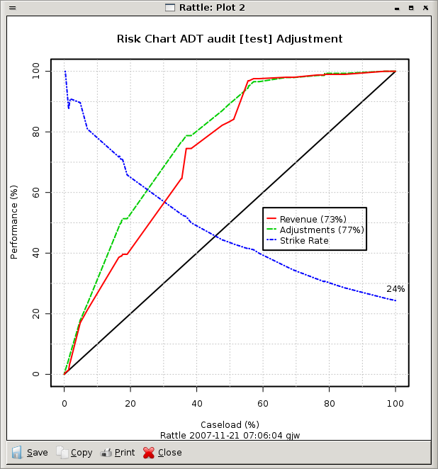
# Plot the results
> pr <- predict(audit.adt, audit[-trainset, c(2:11,13)], type="prob")[,2]
> eval <- evaluateRisk(pr, audit[-trainset, c(2:11,13)]$Adjusted, 
                           audit[-trainset, c(2:11,13,12)]$Adjustment)
> title(main="Risk Chart ADT audit [test] Adjustment", 
        sub=paste("Rattle", Sys.time(), Sys.info()["user"]))

Figure 12.9: Audit risk chart from an alternating decision tree.

() introduced AdaBoost, popularising the idea of ensemble learning where a committee of models cooperate to deliver a better outcome. For a demonstration of AdaBoost visit http://www1.cs.columbia.edu/~freund/adaboost/.

The original formulation of the algorithm, as in (), adjusts all weights each iteration. Weights are increased if the corresponding record is misclassified by $\mathcal{M}_i$ or decreased if it is correctly classified by $\mathcal{M}_i$. The weights are then further normalised each iteration to ensure they continue to represent a distribution (so that $\sum_{j=1}^{n}{w_j}=1$). This can be simplified, as by (), to only increase the weights of the misclassified entities. We use this simpler formulation in the above description of the algorithm. Consequently, the calculation of $\epsilon_i$ (line 9) includes the sum of the weights as a denominator (which is 1 in the original formulation). Only the weights associated with the misclassified entities are modified in line 11. The original algorithm modified all weights by $e^{-\alpha_i y_i \mathcal{M}_i(x_j)}$ which equates to $e^{\alpha_i}$ for misclassified entities (since either $y_i$ or $\mathcal{M}_i(x_j)$ is -1, but not both) and to $e^{-\alpha_i}$ for correctly classified entities (since both $y_i$ or $\mathcal{M}_i(x_j)$ are either 1 or -1). For each iteration the new weights in the original algorithm are normalised by dividing each weight by a calculated factor $Z_i$.

Cost functions other than the exponential loss criterion $e^{-m}$ have been proposed. These include the logistic log-likelihood criterion $\log(1+\exp(-m))$ used in LogitBoost), $1-\tanh(m)$ (Doom II) and $(1-m)I(m>1)$ (Support Vector Machines).

BrownBoost addresses the issue of the sensitivity of AdaBoost to noise.

We note that if each weak classifier is always better than chance, then AdaBoost can be proven to converge to a perfectly accurate model (no training error). Also note that even after achieving an ensemble model with no error, as we add in new models to the ensemble the generalisation error continues to improve (the margin continues to grow). Although it was thought, at first, that AdaBoost does not overfit the data, it has since been shown that it can. However, it generally does not, even for large numbers of iterations.

Extensions to AdaBoost include multi-class classification, application to regression (by transforming the problem into a binary classification task), and localised boosting which is similar to mixtures of experts.

Some early practical work on boosting was undertaken with the Australian Taxation Office using boosted stumps. Multiple, simple models of tax compliance were produced. The models were easily and independently interpretable. Effectively, the models identified a collection of factors that in combination were useful in predicting compliance.

Support further development through the purchase of the PDF version of the book.
The PDF version is a formatted comprehensive draft book (with over 800 pages).
Brought to you by Togaware. This page generated: Wednesday, 19 May 2010